Timing Diagrams

Focusing on time constraints and state changes over a specific timeline.

Timing diagrams in UML 2.5 are specialized behavioral diagrams designed to model precise temporal aspects of system behavior—particularly state changes, value changes, or condition durations over a continuous or discrete timeline. Unlike sequence diagrams (which show discrete message ordering) or state machines (which focus on event-triggered transitions), timing diagrams emphasize time as the primary axis: how long states persist, when transitions must occur, deadlines, periods, jitter, response times, and timing constraints.

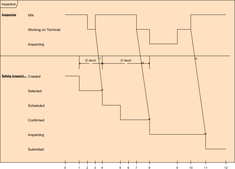
Key elements of timing diagrams:

• Lifeline — Horizontal line for each participant (object, role, component, system, or signal).
• Timeline — Horizontal axis representing time (continuous or discrete ticks).
• State/Condition Timeline — Thick line segment showing duration of a state or value (e.g., solid for “Heating”, dashed for “Idle”).
• Transition — Vertical line or slanted arrow between state changes, labeled with event or trigger.
• Time Constraint — {duration} notation (e.g., {t ≤ 50ms}, {response < 200ms}, {period = 1s ± 10ms}).
• Duration Constraint — Between two points on timeline, e.g., {d} or {min..max}.
• Time Mark — Vertical dashed line labeled t0, t1, etc., for reference points.
• Value Change — Can show variable values over time (e.g., temperature rising from 20°C to 25°C).
• Compact vs. Robust notation — Compact (state line with changes) or robust (explicit state regions).

Timing diagrams are especially valuable in:

• Real-time and embedded systems
• Performance-critical applications
• Protocols with strict timing
• Hardware-software co-design
• Systems with QoS requirements (latency, throughput, jitter)
• Validating SLAs or regulatory timing rules

In Agile & use-case-driven projects, they are used sparingly but powerfully—typically for high-risk timing aspects identified during use case elaboration or architectural spikes.

Practical Examples of Timing Diagrams in Real Projects

Here are numerous concrete examples showing timing diagrams modeling time-sensitive behavior:

• E-commerce – Payment Gateway Response Time SLA
  • Lifelines: :CustomerApp, :PaymentService, :ExternalGateway Timeline: t0 = payment request sent
  • CustomerApp: Processing (t0 to t0+500ms)
  • PaymentService: Authorizing (t0 to t0+200ms) → WaitingForGateway (t0+200ms to t0+800ms)
  • ExternalGateway: Idle → Processing (t0+300ms to t0+700ms) → Approved Constraints: {response time ≤ 1000ms} from t0 to approval {gateway latency ≤ 500ms} Practical benefit: Visualizes end-to-end latency budget; used to set timeouts and retry policies.
• Mobile Banking – Transaction Authorization Timeout
  • Lifelines: :MobileApp, :AuthService, :CoreBanking Timeline: t0 = transfer initiated
  • MobileApp: AwaitingOTP (t0 to t0+120s)
  • AuthService: OTPGenerated → OTPValid (t0 to t0+300s)
  • CoreBanking: Pending → Executed (only if OTP validated within 60s) Constraint: {OTP validity = 120s} Transition at t0+60s: [no OTP entered] → Timeout / cancelTransaction() Practical: Ensures security window is enforced; helps test timeout edge cases.
• Ride-Sharing – ETA Calculation & Real-Time Updates
  • Lifelines: :DriverApp, :MatchingService, :RiderApp Timeline: t0 = ride accepted
  • DriverApp: EnRoute (t0 → t_end) with periodic location updates every 5s ± 1s
  • MatchingService: CalculatingETA (t0 to t0+2s) → StableETA (t0+2s onward)
  • RiderApp: ShowingETA (updates every 10s) Constraint: {ETA refresh ≤ 10s} {jitter ≤ 2s} Practical: Exposes acceptable delay for user experience; guides WebSocket heartbeat frequency.
• Healthcare – Defibrillator Response in Cardiac Arrest
  • Lifelines: :MonitorDevice, :Defibrillator, :Patient Timeline: t0 = arrhythmia detected
  • MonitorDevice: Monitoring → ShockAdvisory (t0 to t0+5s)
  • Defibrillator: Standby → Charging (t0+5s to t0+8s) → ReadyToShock
  • Patient: Fibrillating → NormalRhythm (after shock at t0+10s ± 2s) Constraint: {time to shock ≤ 10s} {charge time ≤ 3s} Practical: Critical for device certification (IEC 60601); used in safety analysis.
• IoT Smart Thermostat – Temperature Control Loop
  • Lifelines: :ThermostatController, :TemperatureSensor, :Heater Timeline: t = continuous
  • TemperatureSensor: Reading (oscillating 19–21°C)
  • ThermostatController: Idle → Heating (when temp < 20°C – 0.5°C hysteresis)
  • Heater: Off → On (duration until temp ≥ 21°C) Constraint: {overshoot ≤ 1°C} {settling time ≤ 5min} {cycle period ≈ 10min} Practical: Models PID-like control loop timing; validates energy efficiency claims.
• Real-Time Stock Trading – Order Matching Latency
  • Lifelines: :TraderGateway, :MatchingEngine, :MarketDataPublisher Timeline: t0 = order arrives
  • TraderGateway: Received → Forwarded (t0 to t0+2ms)
  • MatchingEngine: Queued → Matching (t0+2ms to t0+5ms) → Executed
  • MarketDataPublisher: UpdateSent (within t0+10ms) Constraint: {end-to-end matching ≤ 5ms} {market data update ≤ 10ms} Practical: Regulatory requirement visualization; used in performance budgeting.
• Automotive – Adaptive Cruise Control Reaction
  • Lifelines: :RadarSensor, :ACCController, :ThrottleActuator, :BrakeActuator Timeline: t0 = lead vehicle slows
  • RadarSensor: Detecting → RangeDecreasing
  • ACCController: Maintaining → Decelerating (t0+50ms)
  • ThrottleActuator: Open → Closing (t0+100ms)
  • BrakeActuator: Inactive → LightBraking (t0+200ms if needed) Constraint: {reaction time ≤ 200ms} {deceleration ramp ≤ 3m/s²} Practical: ISO 26262 safety timing analysis; shows coordinated actuator response.
• Embedded Device – Watchdog Timer Reset
  • Lifelines: :Application, :WatchdogTimer Timeline: t = continuous
  • Application: Running → Stalled (if no kick within 500ms)
  • WatchdogTimer: Armed → Timeout (after 500ms) → ResetSystem Constraint: {kick interval ≤ 400ms} {tolerance ±50ms} Practical: Ensures system recovery from hangs; critical for reliability in field devices.

In Visual Paradigm:

• Create horizontal lifelines and drag state/condition segments.
• Add time constraints with curly braces {…}.
• Use compact mode for simple state changes or robust for detailed durations.
• Annotate with time marks (t0, t1) and duration markers.
• Simulate timing to verify constraints.
• Semantic backplane links timing constraints to state machines, sequence messages, or requirements.

Timing diagrams are the precision instrument for time-critical behavior—making deadlines, latencies, periods, and jitter explicit and verifiable. They complete the set of 7 behavioral diagrams, equipping you to model both high-level orchestration and microsecond-level timing constraints.

With the heartbeat of behavior fully covered, you’re ready for Module 5: Agile Architecture and Implementation Workflows, where we connect everything to code, patterns, and iterative delivery.